MNIST tutorial

Welcome to Flax NNX! In this tutorial you will learn how to build and train a simple convolutional neural network (CNN) to classify handwritten digits on the MNIST dataset using the Flax NNX API.

Flax NNX is a Python neural network library built upon JAX. If you have used the Flax Linen API before, check out Why Flax NNX. You should have some knowledge of the main concepts of deep learning.

Let’s get started!

1. Install Flax

If flax is not installed in your Python environment, use pip to install the package from PyPI (below, just uncomment the code in the cell if you are working from Google Colab/Jupyter Notebook):

# !pip install -U "jax[cuda12]"
# !pip install -U flax

2. Load the MNIST dataset

First, you need to load the MNIST dataset and then prepare the training and testing sets via Tensorflow Datasets (TFDS). You normalize image values, shuffle the data and divide it into batches, and prefetch samples to enhance performance.

import tensorflow_datasets as tfds  # TFDS to download MNIST.
import tensorflow as tf  # TensorFlow / `tf.data` operations.

tf.random.set_seed(0)  # Set the random seed for reproducibility.

train_steps = 1200
eval_every = 200
batch_size = 32

train_ds: tf.data.Dataset = tfds.load('mnist', split='train')
test_ds: tf.data.Dataset = tfds.load('mnist', split='test')

train_ds = train_ds.map(
  lambda sample: {
    'image': tf.cast(sample['image'], tf.float32) / 255,
    'label': sample['label'],
  }
)  # normalize train set
test_ds = test_ds.map(
  lambda sample: {
    'image': tf.cast(sample['image'], tf.float32) / 255,
    'label': sample['label'],
  }
)  # Normalize the test set.

# Create a shuffled dataset by allocating a buffer size of 1024 to randomly draw elements from.
train_ds = train_ds.repeat().shuffle(1024)
# Group into batches of `batch_size` and skip incomplete batches, prefetch the next sample to improve latency.
train_ds = train_ds.batch(batch_size, drop_remainder=True).take(train_steps).prefetch(1)
# Group into batches of `batch_size` and skip incomplete batches, prefetch the next sample to improve latency.
test_ds = test_ds.batch(batch_size, drop_remainder=True).prefetch(1)

3. Define the model with Flax NNX

Create a CNN for classification with Flax NNX by subclassing nnx.Module:

from flax import nnx  # The Flax NNX API.
from functools import partial
from typing import Optional

class CNN(nnx.Module):
  """A simple CNN model."""

  def __init__(self, *, rngs: nnx.Rngs):
    self.conv1 = nnx.Conv(1, 32, kernel_size=(3, 3), rngs=rngs)
    self.batch_norm1 = nnx.BatchNorm(32, rngs=rngs)
    self.dropout1 = nnx.Dropout(rate=0.025)
    self.conv2 = nnx.Conv(32, 64, kernel_size=(3, 3), rngs=rngs)
    self.batch_norm2 = nnx.BatchNorm(64, rngs=rngs)
    self.avg_pool = partial(nnx.avg_pool, window_shape=(2, 2), strides=(2, 2))
    self.linear1 = nnx.Linear(3136, 256, rngs=rngs)
    self.dropout2 = nnx.Dropout(rate=0.025)
    self.linear2 = nnx.Linear(256, 10, rngs=rngs)

  def __call__(self, x, rngs: nnx.Rngs | None = None):
    x = self.avg_pool(nnx.relu(self.batch_norm1(self.dropout1(self.conv1(x), rngs=rngs))))
    x = self.avg_pool(nnx.relu(self.batch_norm2(self.conv2(x))))
    x = x.reshape(x.shape[0], -1)  # flatten
    x = nnx.relu(self.dropout2(self.linear1(x), rngs=rngs))
    x = self.linear2(x)
    return x

# Instantiate the model.
model = CNN(rngs=nnx.Rngs(0))
# Visualize it.
nnx.display(model)

Run the model

Let’s put the CNN model to the test! Here, you’ll perform a forward pass with arbitrary data and print the results.

import jax.numpy as jnp  # JAX NumPy

y = model(jnp.ones((1, 28, 28, 1)), nnx.Rngs(0))
y

Array([[ 0.11409501,  0.4546129 , -0.6421267 , -0.12122799, -0.22859162,
         0.13616608,  1.0126765 , -0.03625144,  0.6132787 , -0.06018351]],      dtype=float32)

4. Create the optimizer and define some metrics

In Flax NNX, you need to create an nnx.Optimizer object to manage the model’s parameters and apply gradients during training. nnx.Optimizer receives the model’s reference, so that it can update its parameters, and an Optax optimizer to define the update rules. Additionally, you will define an nnx.MultiMetric object to keep track of the Accuracy and the Average loss.

import optax

learning_rate = 0.005
momentum = 0.9

optimizer = nnx.Optimizer(
  model, optax.adamw(learning_rate, momentum), wrt=nnx.Param
)
metrics = nnx.MultiMetric(
  accuracy=nnx.metrics.Accuracy(),
  loss=nnx.metrics.Average('loss'),
)

nnx.display(optimizer)

5. Define training step functions

In this section, you will define a loss function using the cross entropy loss (optax.softmax_cross_entropy_with_integer_labels()) that the CNN model will optimize over.

In addition to the loss, during training and testing you will also get the logits, which will be used to calculate the accuracy metric.

During training — the train_step — you will use nnx.value_and_grad to compute the gradients and update the model’s parameters using the optimizer you have already defined. The train_step also receives an nnx.Rngs object to provide randomness for dropout. The eval_step omits rngs because the eval view already has deterministic=True, so dropout is disabled and no random key is needed. During both steps, the loss and logits are used to update the metrics.

def loss_fn(model: CNN, batch, rngs: nnx.Rngs | None = None):
  logits = model(batch['image'], rngs)
  loss = optax.softmax_cross_entropy_with_integer_labels(
    logits=logits, labels=batch['label']
  ).mean()
  return loss, logits

@nnx.jit
def train_step(model: CNN, optimizer: nnx.Optimizer, metrics: nnx.MultiMetric, rngs: nnx.Rngs, batch):
  """Train for a single step."""
  grad_fn = nnx.value_and_grad(loss_fn, has_aux=True)
  (loss, logits), grads = grad_fn(model, batch, rngs)
  metrics.update(loss=loss, logits=logits, labels=batch['label'])  # In-place updates.
  optimizer.update(model, grads)  # In-place updates.

@nnx.jit
def eval_step(model: CNN, metrics: nnx.MultiMetric, batch):
  loss, logits = loss_fn(model, batch)
  metrics.update(loss=loss, logits=logits, labels=batch['label'])  # In-place updates.

In the code above, the nnx.jit transformation decorator traces the train_step function for just-in-time compilation with XLA, optimizing performance on hardware accelerators, such as Google TPUs and GPUs. nnx.jit is a stateful version of the jax.jit transform that allows its function input and outputs to be Flax NNX objects. Similarly, nnx.value_and_grad is a stateful version of jax.value_and_grad. Check out the transforms guide to learn more.

Note: The code shows how to perform several in-place updates to the model, the optimizer, the RNG streams, and the metrics, but state updates were not explicitly returned. This is because Flax NNX transformations respect reference semantics for Flax NNX objects, and will propagate the state updates of the objects passed as input arguments. This is a key feature of Flax NNX that allows for a more concise and readable code. You can learn more in Why Flax NNX.

6. Train and evaluate the model

Now, you can train the CNN model. Before the training loop, we use nnx.view to create a train_model (with dropout enabled and batch norm in training mode) and an eval_model (with dropout disabled and batch norm using running statistics). These views share the same underlying weights, so updates during training are automatically reflected during evaluation.

from IPython.display import clear_output
import matplotlib.pyplot as plt

metrics_history = {
  'train_loss': [],
  'train_accuracy': [],
  'test_loss': [],
  'test_accuracy': [],
}

rngs = nnx.Rngs(0)
train_model = nnx.view(model, deterministic=False, use_running_average=False)
eval_model = nnx.view(model, deterministic=True, use_running_average=True)

for step, batch in enumerate(train_ds.as_numpy_iterator()):
  # Run the optimization for one step and make a stateful update to the following:
  # - The train state's model parameters
  # - The optimizer state
  # - The training loss and accuracy batch metrics
  train_step(train_model, optimizer, metrics, rngs, batch)

  if step > 0 and (step % eval_every == 0 or step == train_steps - 1):  # One training epoch has passed.
    # Log the training metrics.
    for metric, value in metrics.compute().items():  # Compute the metrics.
      metrics_history[f'train_{metric}'].append(value)  # Record the metrics.
    metrics.reset()  # Reset the metrics for the test set.

    # Compute the metrics on the test set after each training epoch.
    for test_batch in test_ds.as_numpy_iterator():
      eval_step(eval_model, metrics, test_batch)

    # Log the test metrics.
    for metric, value in metrics.compute().items():
      metrics_history[f'test_{metric}'].append(value)
    metrics.reset()  # Reset the metrics for the next training epoch.

    clear_output(wait=True)
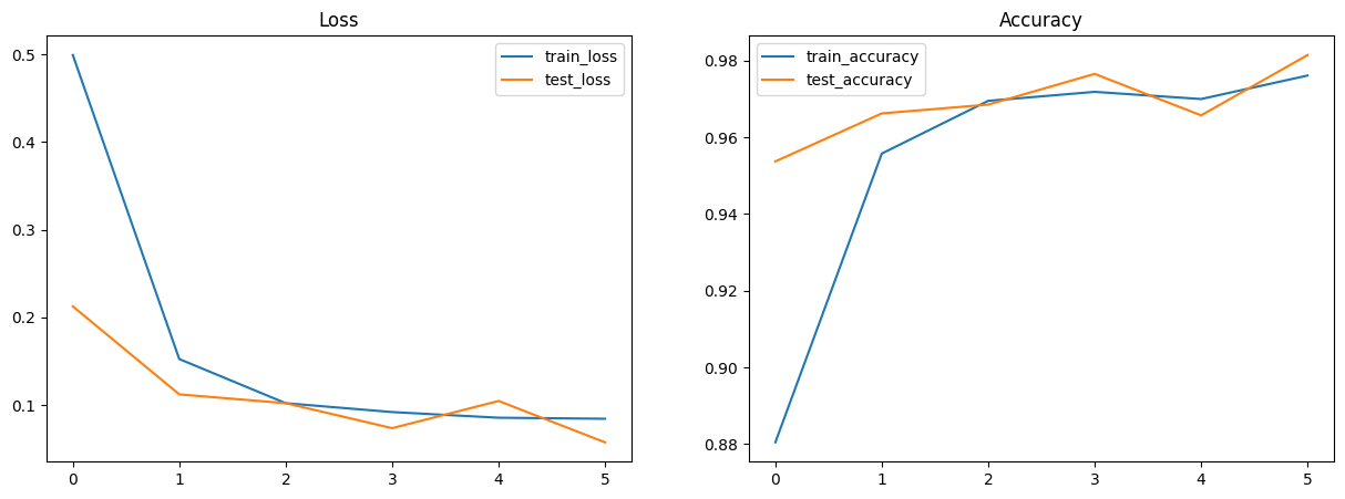
    # Plot loss and accuracy in subplots
    fig, (ax1, ax2) = plt.subplots(1, 2, figsize=(15, 5))
    ax1.set_title('Loss')
    ax2.set_title('Accuracy')
    for dataset in ('train', 'test'):
      ax1.plot(metrics_history[f'{dataset}_loss'], label=f'{dataset}_loss')
      ax2.plot(metrics_history[f'{dataset}_accuracy'], label=f'{dataset}_accuracy')
    ax1.legend()
    ax2.legend()
    plt.show()

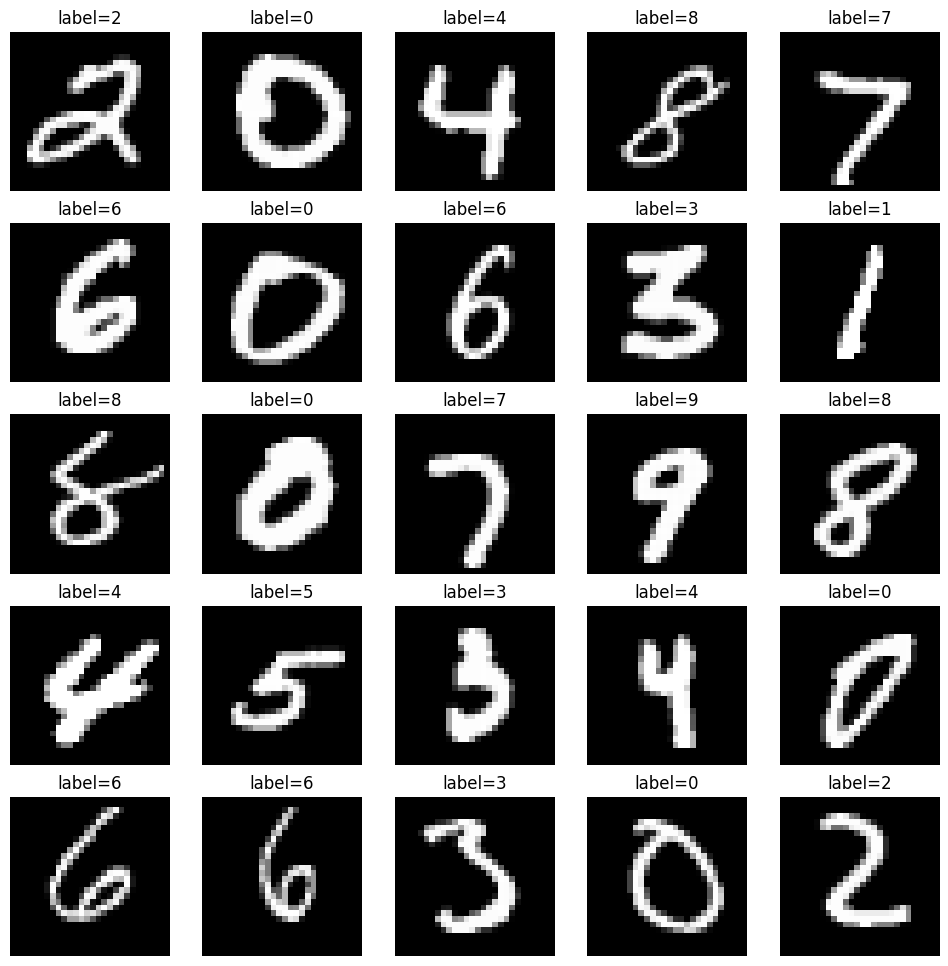
7. Perform inference on the test set

Create a jit-compiled model inference function (with nnx.jit) - pred_step - to generate predictions on the test set using the learned model parameters. Since we already have eval_model (an nnx.view with deterministic=True and use_running_average=True), we can use it directly for inference. This will enable you to visualize test images alongside their predicted labels for a qualitative assessment of model performance.

@nnx.jit
def pred_step(model: CNN, batch):
  logits = model(batch['image'], None)
  return logits.argmax(axis=1)

We reuse the eval_model view created earlier so that Dropout is disabled and BatchNorm uses stored running stats during inference.

test_batch = test_ds.as_numpy_iterator().next()
pred = pred_step(eval_model, test_batch)

fig, axs = plt.subplots(5, 5, figsize=(12, 12))
for i, ax in enumerate(axs.flatten()):
  ax.imshow(test_batch['image'][i, ..., 0], cmap='gray')
  ax.set_title(f'label={pred[i]}')
  ax.axis('off')

8. Export the model

Flax models are great for research, but aren’t meant to be deployed directly. Instead, high performance inference runtimes like LiteRT or TensorFlow Serving operate on a special SavedModel format. The Orbax library makes it easy to export Flax models to this format. First, we must create a JaxModule object wrapping a model and its prediction method.

from orbax.export import JaxModule, ExportManager, ServingConfig

def exported_predict(model, y):
    return model(y, None)

jax_module = JaxModule(eval_model, exported_predict)

We also need to tell Tensorflow Serving what input type exported_predict expects in its second argument. The export machinery expects type signature arguments to be PyTrees of tf.TensorSpec.

sig = [tf.TensorSpec(shape=(1, 28, 28, 1), dtype=tf.float32)]

Finally, we can bundle up the input signature and the JaxModule together using the ExportManager class.

export_mgr = ExportManager(jax_module, [
    ServingConfig('mnist_server', input_signature=sig)
])

output_dir='/tmp/mnist_export'
export_mgr.save(output_dir)

Congratulations! You have learned how to use Flax NNX to build and train a simple classification model end-to-end on the MNIST dataset.

Next, check out Why Flax NNX? and get started with a series of Flax NNX Guides.